Joined Dataflow Example

The example provide quick walkthrough of how to aggregate and prepare data for Machine Learning using Amazon SageMaker Data Wrangler for joined dataset.

Music Recommendation Example

With the rapid growth of the commercial music streaming services, more and more people nowadayas are listening to music from they model devices. However, organising, managing and searching among all the digital music produced by the society is a very time-cosuming and tedious task. Using a music recommender system to predict the user’s choices and suggest songs that is likely to be interesting has been a common practice used by the music providers.

Background

Amazon SageMaker helps data scientists and developers to prepare, build, train, and deploy machine learning models quickly by bringing together a broad set of purpose-built capabilities. This example shows how SageMaker can accelerate machine learning development during the data preprocessing stage to help build the musical playlist tailored to a user’s tastes.

Dataset

Dataset

The dataset is required before we begin, ensure that you have downloaded it by following the instructions below.

Example track (track.csv) and user ratings (ratings.csv) data is provided on a publicly available S3 bucket found here: s3://sagemaker-sample-files/datasets/tabular/synthetic-music We’ll be running a notebook to download the data in the demo so no need to manually download it from here just yet.

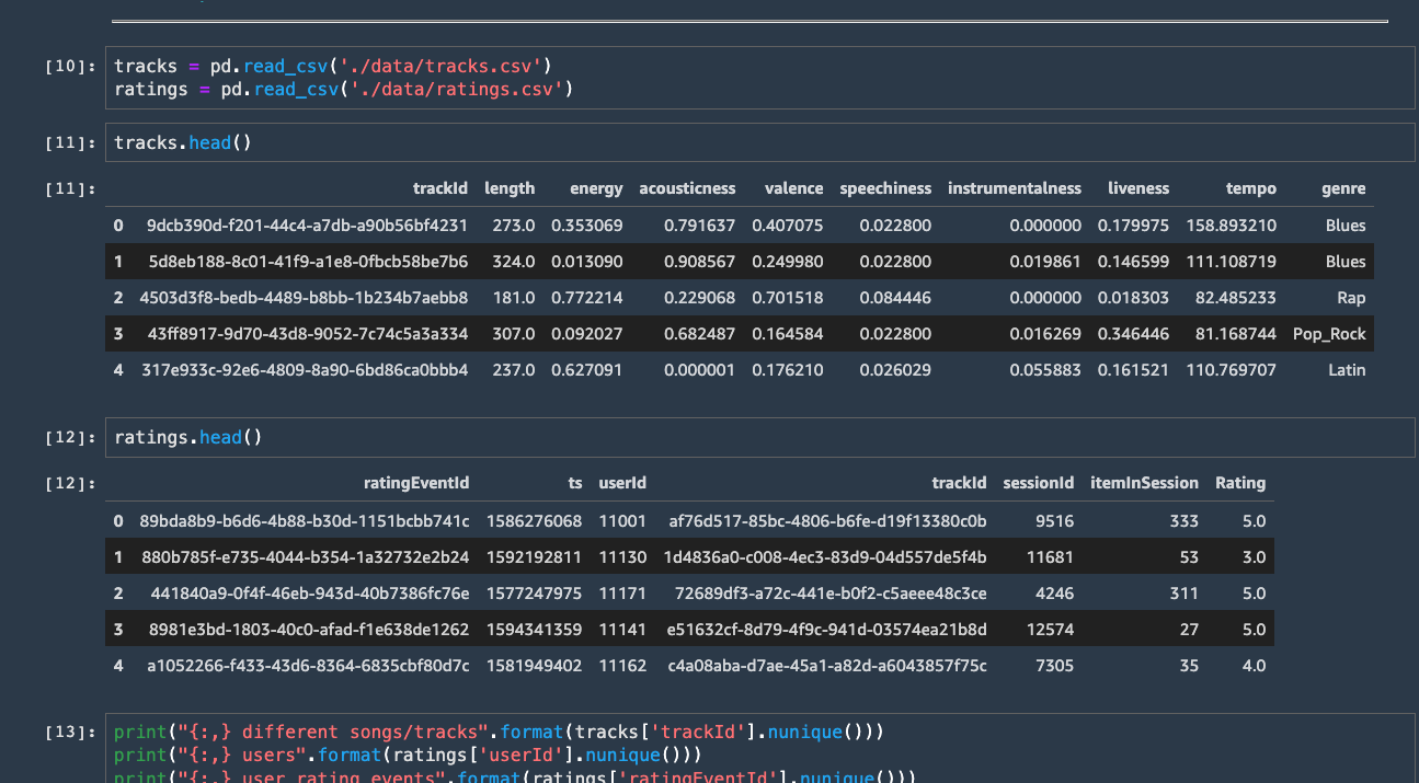
tracks.csv

Column name	Description
trackId	unique identifier for each song/track
length	song length in seconds (numerical)
energy	Energy is a measure from 0.0 to 1.0 and represents a perceptual measure of intensity and activity (numerical)
acousticness	A confidence measure from 0.0 to 1.0 of whether the track is acoustic. (numerical)
valence	A measure from 0.0 to 1.0 describing the musical positiveness conveyed by a track. (numerical)
speechiness	Speechiness detects the presence of spoken words in a track. (numerical)
instrumentalness	Predicts whether a track contains no vocals. (numerical)
liveness	Detects the presence of an audience in the recording. (numerical)
tempo	The overall estimated tempo of a track in beats per minute (BPM). (numerical)
genre	The genre of the song. For example, pop, rock etc. (categorical)

ratings.csv

Column name	Description
ratingEventId	unique identifier for each rating
ts	timestamp of rating event (datetime in seconds since 1970)
userId	unique id for each user
trackId	unique id for each song/track
sessionId	unique id for the user’s session
Rating	user’s rating of song on scale from 1 to 5

For this example, we’ll be using our own generated track and user ratings data, but publicly available datasets/apis such as the Million Song Dataset and open-source song ratings APIs are available for personal research purposes. A full end-to-end pipeline can be found in this SageMaker example.

Pre-requisites:

We need to ensure dataset (tracks and ratings dataset) for ML is uploaded to a data source (instructions to download the dataset to Amazon S3 is available in the following section). Data source can be any one of the following options:

• S3

• Athena

• RedShift

• SnowFlake

Data Source

For this experiment the Data Source will be Amazon S3

Experiment steps

Downloading the dataset, and notebooks

Ensure that you have a working Amazon SageMaker Studio environment and that it has been updated.

Follow the steps below to download the dataset.

Start with the explore-dataset.ipynb SageMaker Studio notebook.

• Explore the dataset locally by running the cells in the

notebook. * Upload the datasets (CSV files) to an S3 location for consumption by SageMaker Data Wrangler later. * Copy the S3 URLs of the tracks and ratings data files to your clipboard. We will use these URLs later to import these part files into Data Wrangler and join them.

Let’s run though each of the steps above.

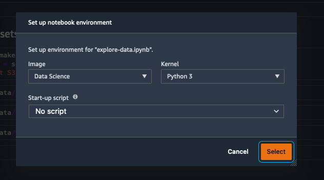
Double click on the file called explore-data.ipynb. Amazon SageMaker may prompt you to select a kernel and image. If it does select Data Science as the image and Python 3 as the Kernel, as shown here:

You have now successfully downloaded the data and opened a notebook, we will now upload the data to your S3 bucket. Note: An Amazon S3 bucket was created for you when the Amazon SageMaker Studio environment was started.

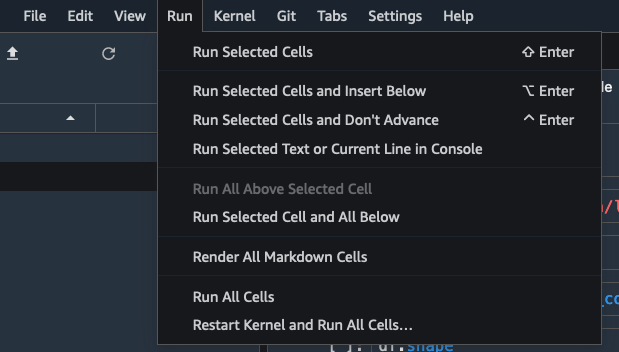
From the menu select Run / Run All Cells to execute all the cells in the notebook.

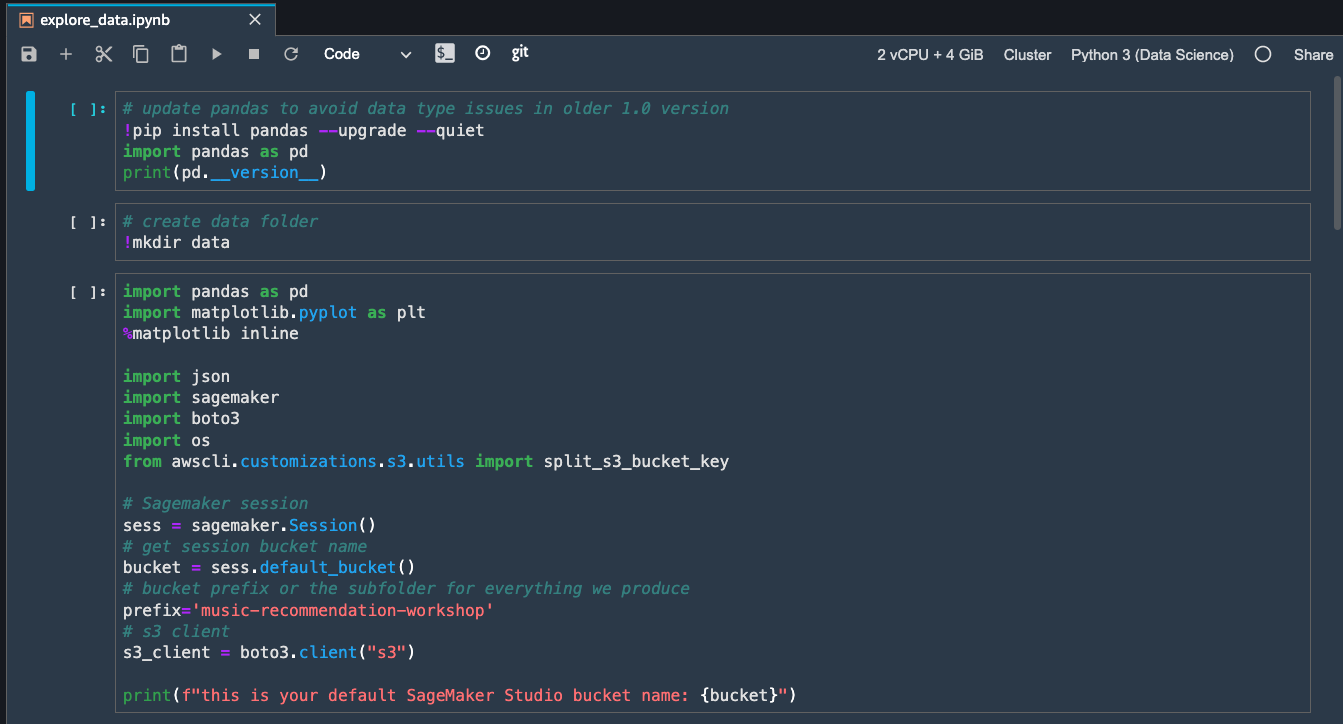
Examine the results, as you can see the samples of the data are printed to the screen.

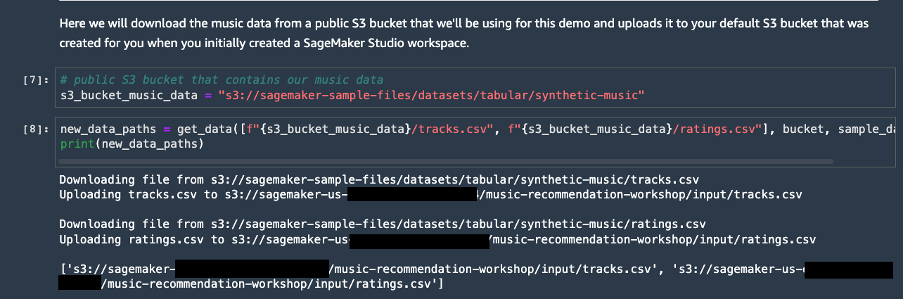
The data structure is defined in the next section. However, before we continue, note the path to the various datasets. Your paths will be different to the ones in the image below. Please copy these paths as you will use them later. An example of a path is s3://sagemaker-eu-west-1-112233445566/music-recommendation-demo/input/tracks.csv

Note

Please also check the S3 location to make sure the files are uploaded successfully before moving to the next section.

In the next section we will import the datasets into Data Wrangler via the SageMaker Studio User Interface (UI).

Importing datasets from a data source (S3) to Data Wrangler

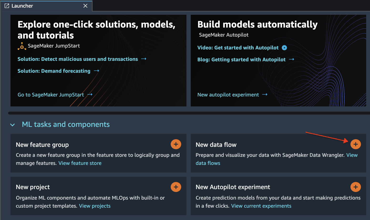
Initialize SageMaker Data Wrangler via SageMaker Studio UI.

There are two ways that you can do this, either from the Launcher screen as depicted here:

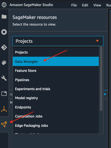
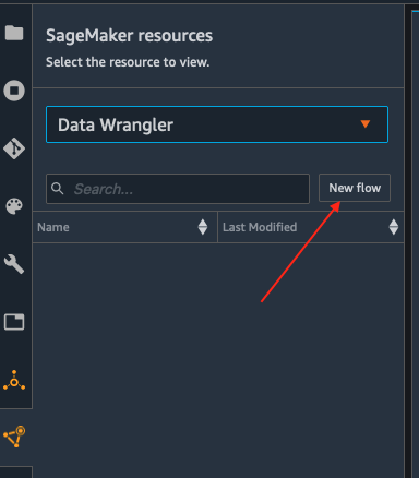
Or from the SageMaker resources menu on the left, selecting Data Wrangler, and new flow

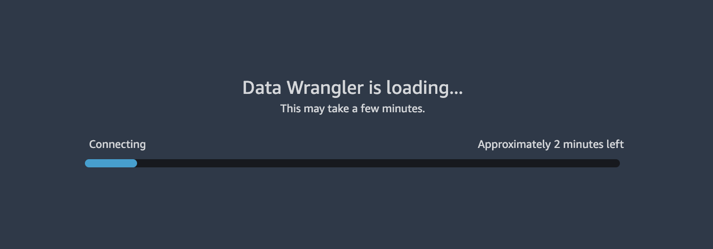
It takes a few minutes to load.

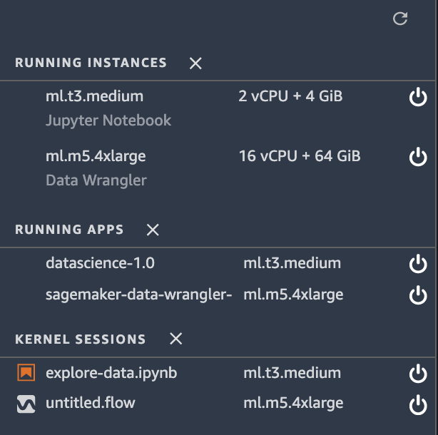
Once Data Wrangler is loaded, you should be able to see it under running instances and apps as shown below.

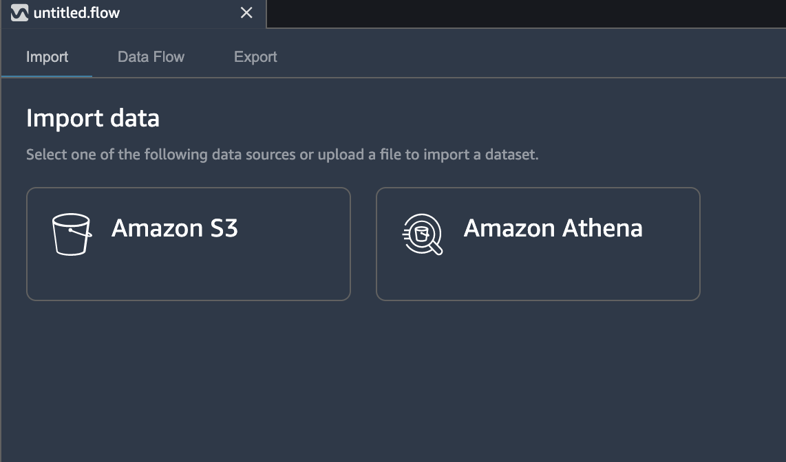
Next, make sure you have copied the data paths when running the explore_data.ipynb notebook from the previous section (see section: Downloading the dataset, and notebooks), as you will need them in this section. Once Data Wrangler is up and running, you can see the following data flow interface with options for import, creating data flows and export as shown below.

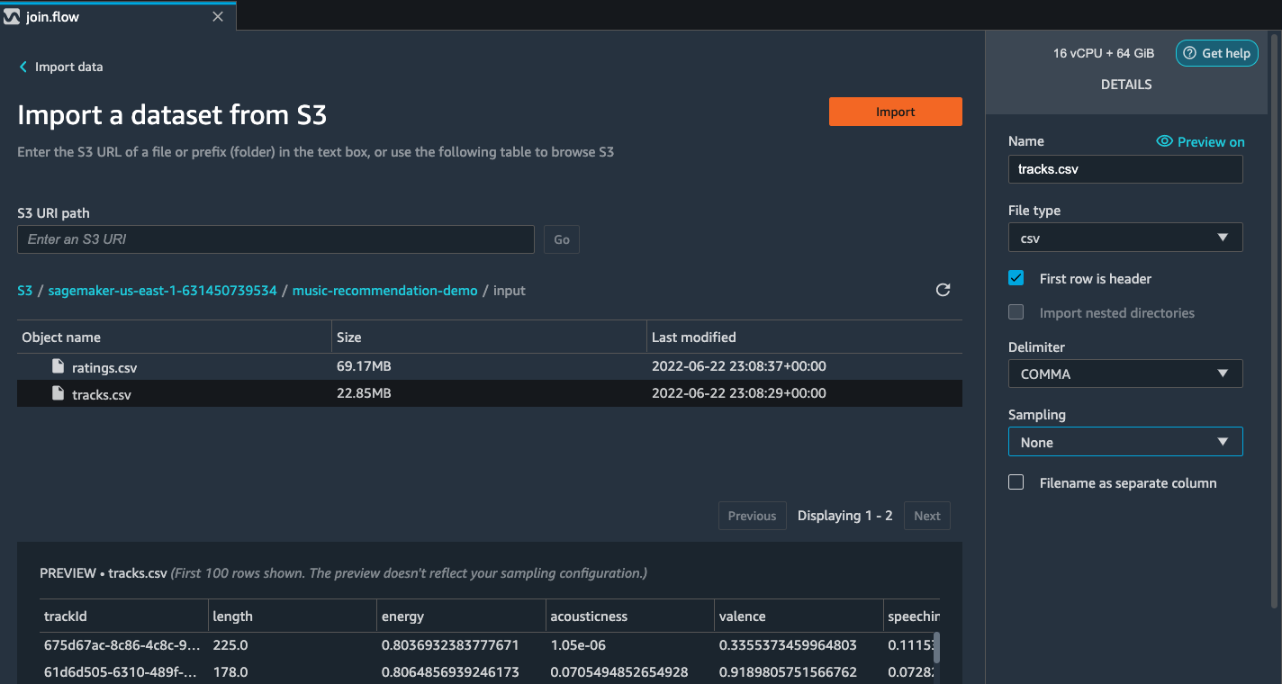
Make sure to rename the untitled.flow to your preference (for e.g., join.flow) Paste the S3 URL for the tracks.csv file into the search box below and hit go.

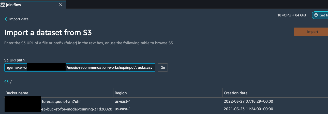
Select the CSV file from the drop down results. On the right pane, make sure COMMA is chosen as the delimiter and Sampling is None. Hit import to import this dataset to Data Wrangler.

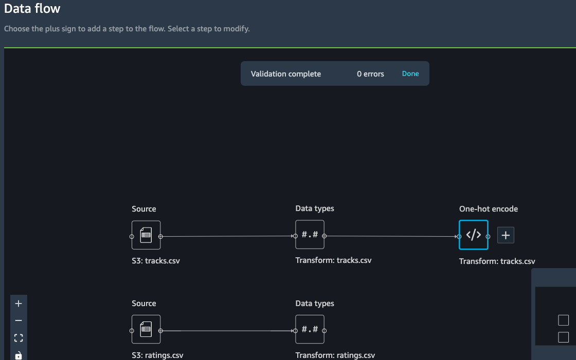
Once the dataset is imported, the Data flow interface looks as shown below.

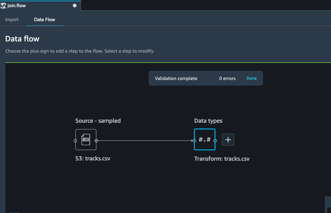
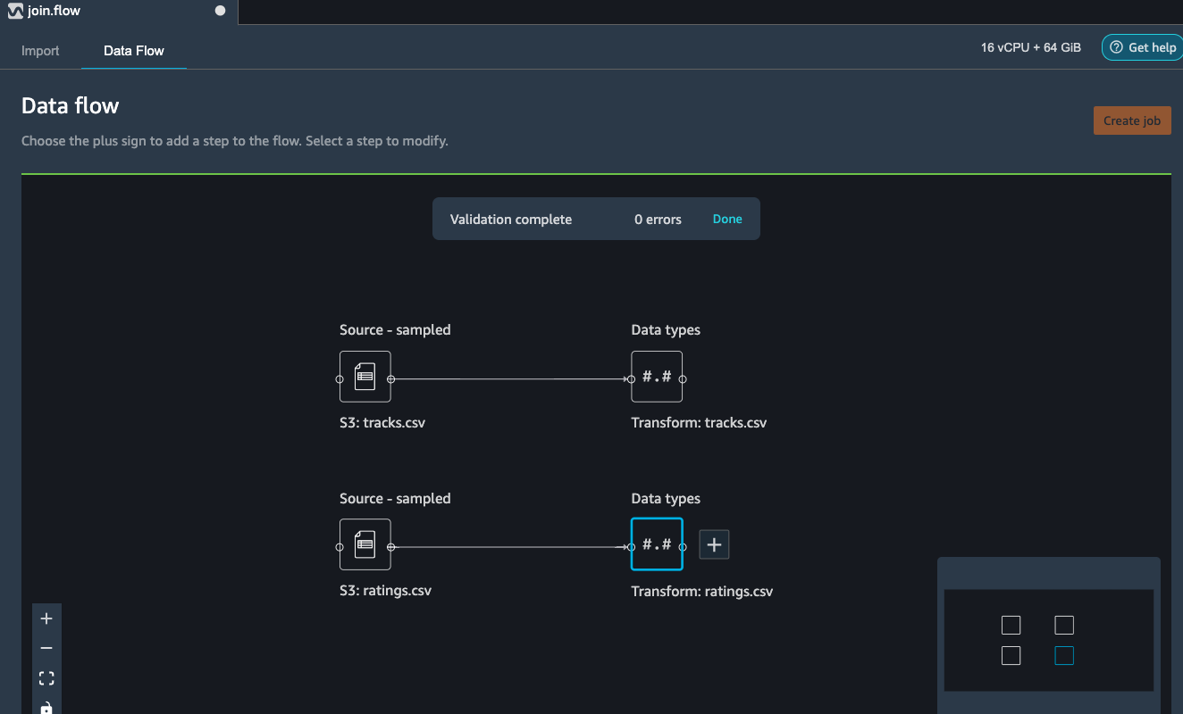
Since currently you are in the data flow tab, hit the import tab (left of data flow tab) as seen in the above image. Import the second part file (ratings.csv) following the same set of instructions as noted previously.

Transform tracks dataset

We firstly want to perform some data transformation using Data Wrangler. Let us walkthough how to perform different transformations using built-in and custom formula functionality in Data Wrangler.

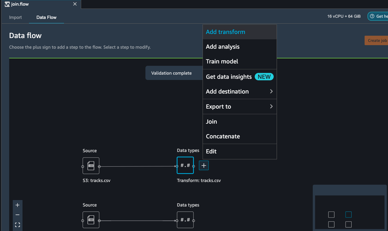
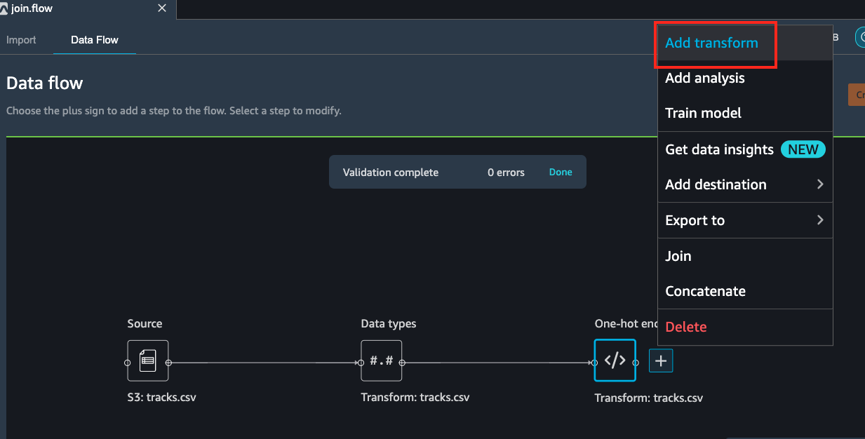
As the genre column in the tracks dataset is a categorical feature, we need to perform one-hot encoding to trasform this feature. Click on the tracks file transform block as show in the image below and select Add transform:

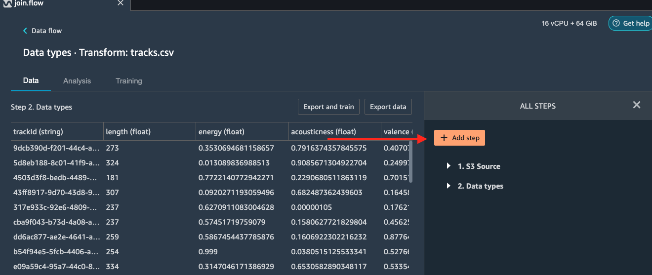
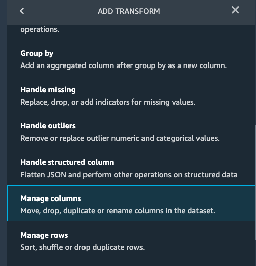
This takes us to the Data Wrangler transformations interface where there are over 300+ transformations you can apply to your dataset. Select Add step as shown below.

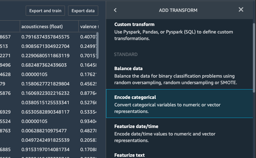
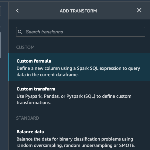
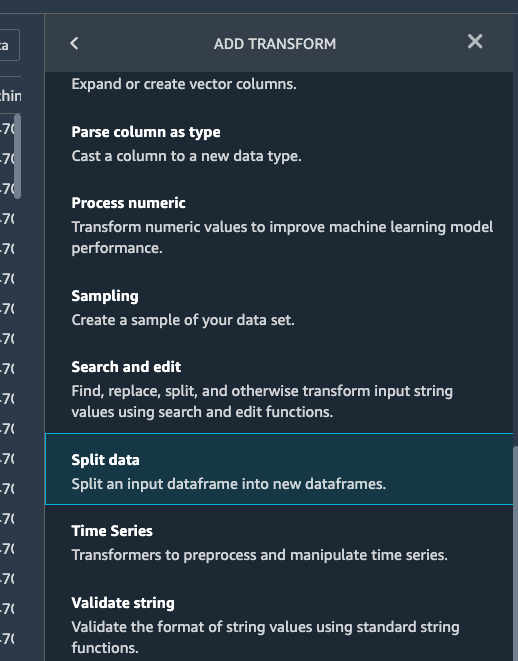
In the ADD TRANFORM window, double click the option Encode categorical.

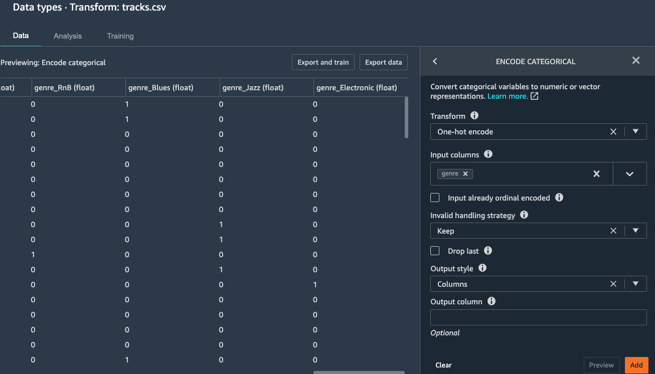
Then on the ENCODE CATEGORICAL window, choose One-hot encode as the Transform type, genre as the input columns, and Columns as the output style. Click Preview and the output is shown as below:

Click Add to add the tranform step to the flow. If you go back to the Data Flow, you can see the step has been added.

We also want to generate a new feature based on the danceability of the track. Danceability describes how suitable a track is for dancing based on a combination of musical elements including tempo, rhythm stability, beat strength, and overall regularity.

• Click on the newly added One-hot encode step and select *Add

transformation*:

Select Add step and choose Custom formula.

Copy and paste below formula and put danceability to the Output Column.

0.3*valence + 0.1*liveness + 0.1*energy

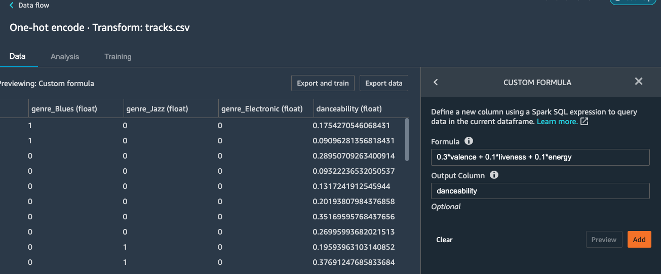
Click Preview and Add the step to the flow.

Joining datasets - first join

Given, we have imported both the tracks and ratings CSV files in the beginning steps. Let us walk through on how to join these CSV files based on a common unique identifier column, trackId. Then we will perform some feature engineering to generate a new set of features that can help to enrich the trainig data.

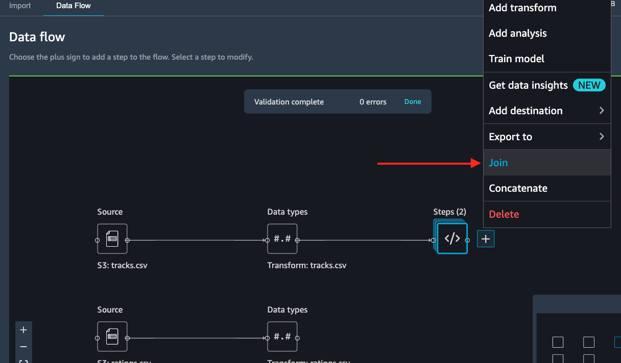
Click on either the tracks or ratings transform block as shown in the image blow:

Here, we have selected tracks transform flow block and hit Join

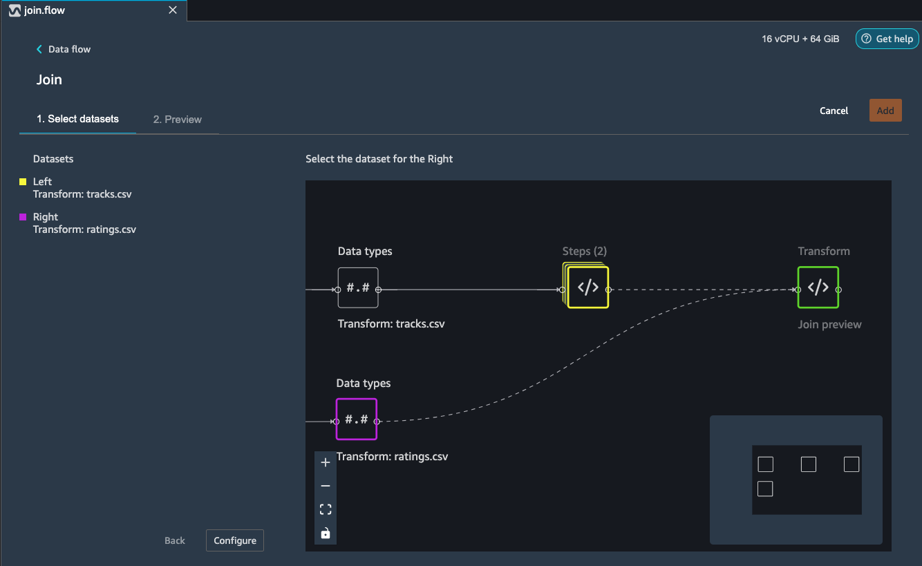
Select the other rating file transform block and it automatically maps (converges) both the files into a Join preview as shown below.

Note Files can also be concatenated similar to join operations .. raw:: html

Hit configure.

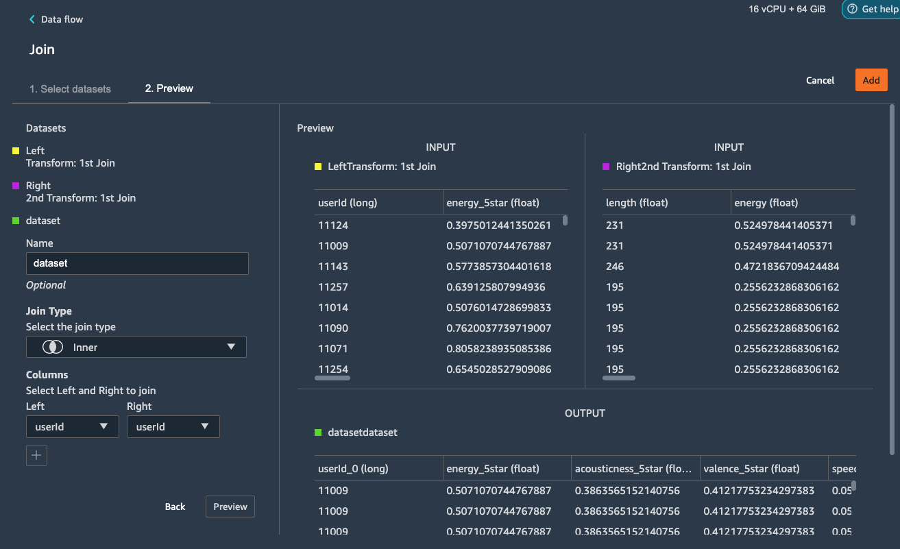
Here, choose a name for the resulting join file and choose the type of join and columns on to join (Please refer to the image below).

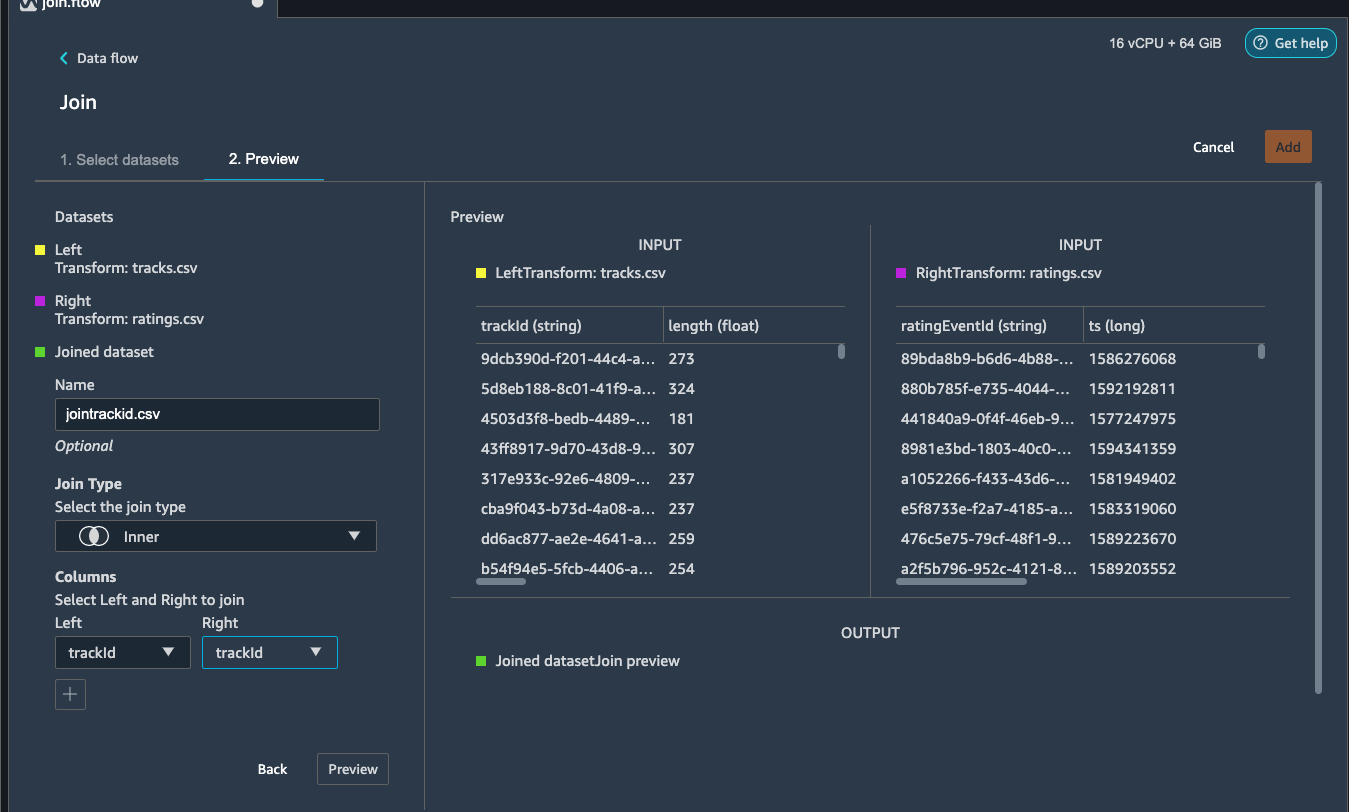
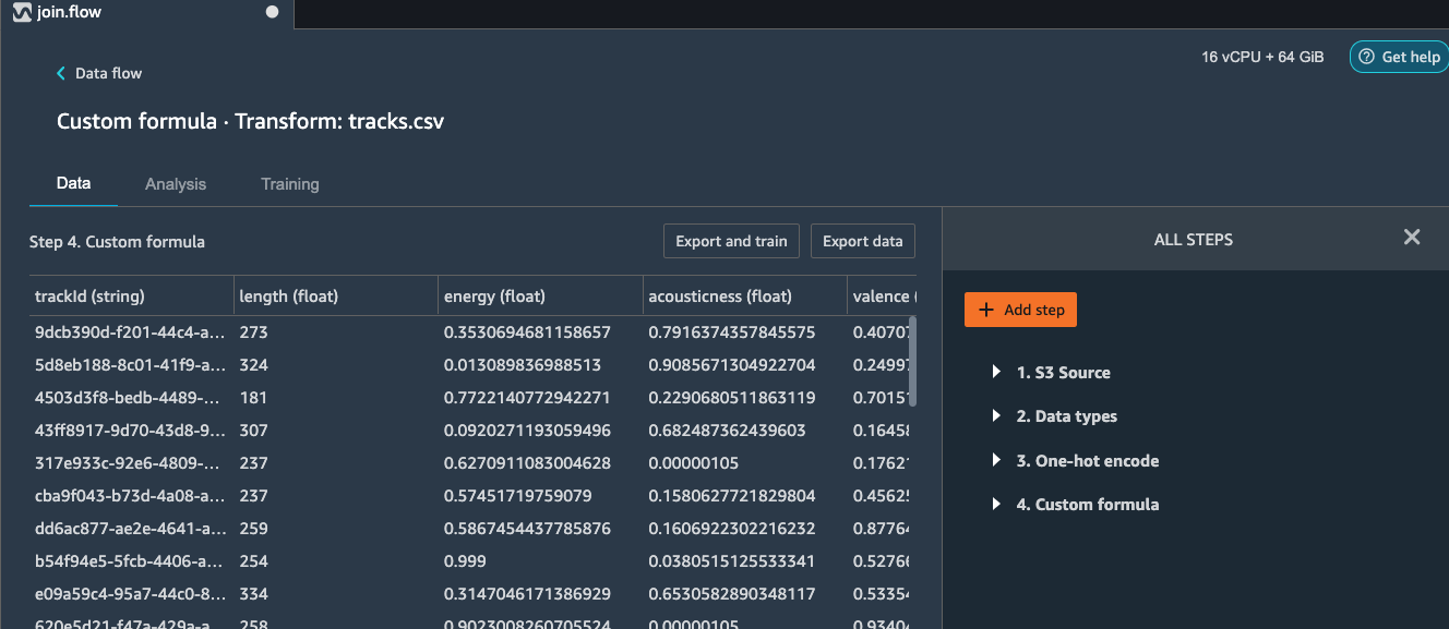
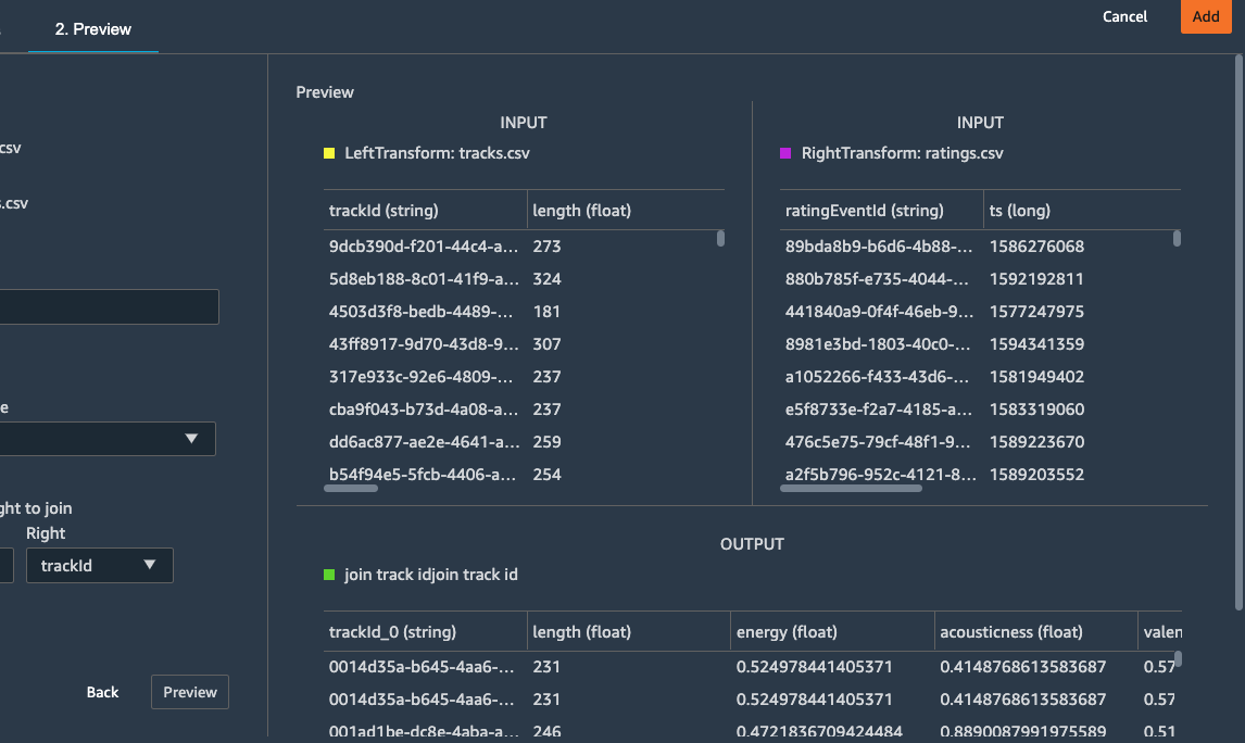
Hit Apply (Preview) . You can see a preview of the Joined dataset as shown in the image below.

Note

Depending on the version of SageMaker it might be Preview and not Add

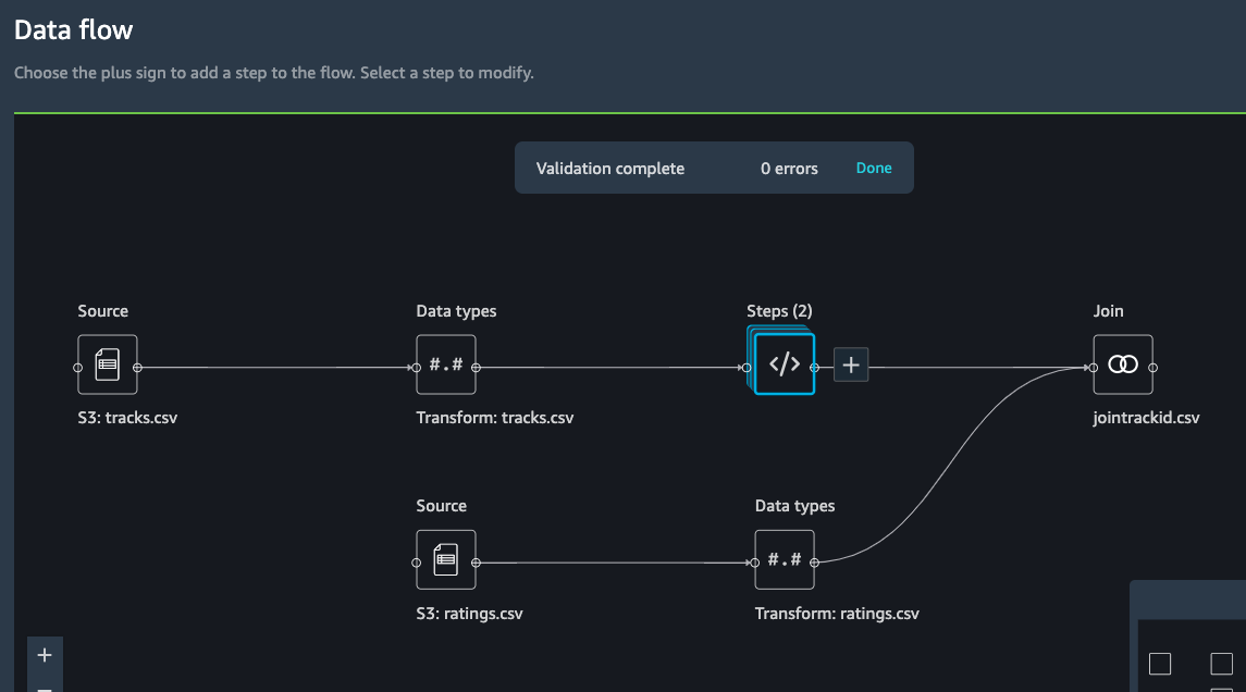
Hit Add at the upper right corner to add this Join transform to the original data flow.

At the end of this step, the data flow looks as shown below.

Next step, let’s see how to use Data Wrangler to add custom transform to perform more advanced feature engineering. Here, we want to use pyspark to calculate the average values of 5-star ratings for different columns and use them as new features.

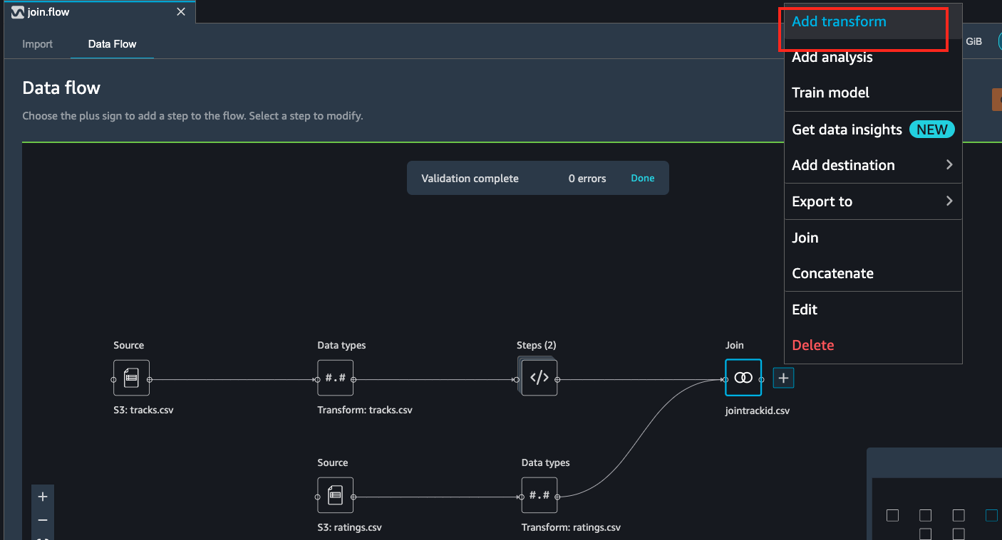
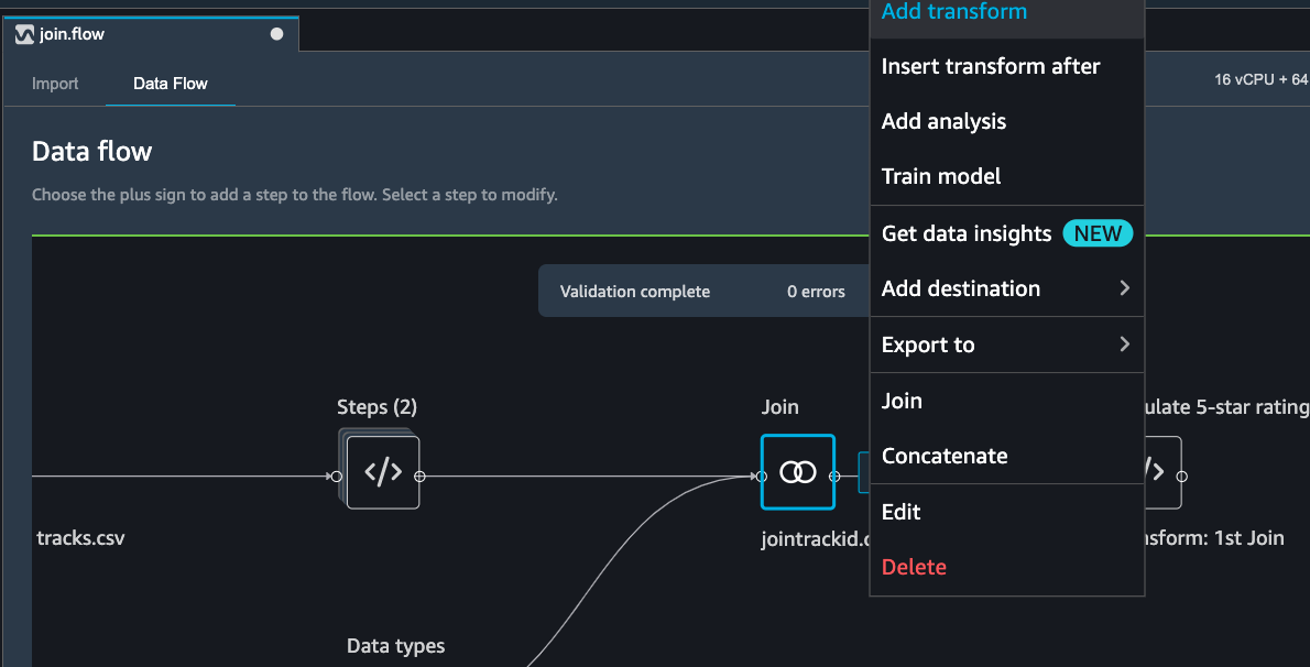
Select on the jointrackid.csv block and click the + icon, under which click on Add transform.

Click the custom transform at this step.

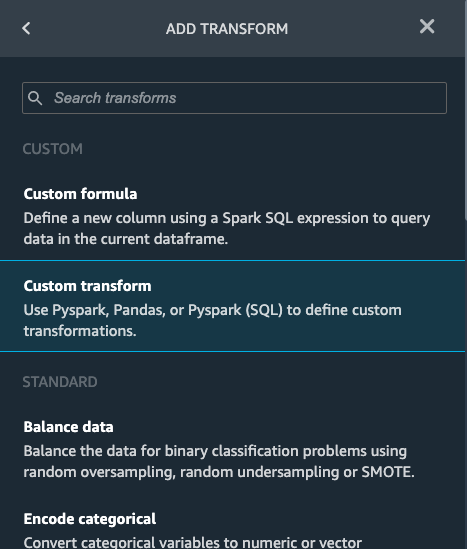
Give a name to this custom transform step and copy and paste below custom script to the window.

# Table is available as variable `df`
import pyspark.sql.functions as F
# numeric features
num_feat_cols = ['energy', 'acousticness', 'valence', 'speechiness', 'instrumentalness', 'liveness', 'tempo', 'danceability', 'genre_Latin', 'genre_Folk',  'genre_Blues', 'genre_Rap', 'genre_Reggae', 'genre_Jazz', 'genre_RnB', 'genre_Country', 'genre_Electronic', 'genre_Pop_Rock']
# calculate averages for 5-star ratings
agg_obj = [F.avg(feat_col).alias(feat_col+"_5star") for feat_col in num_feat_cols]
df = df.filter(F.col('Rating')==5).groupBy('userId').agg(*agg_obj)

• 

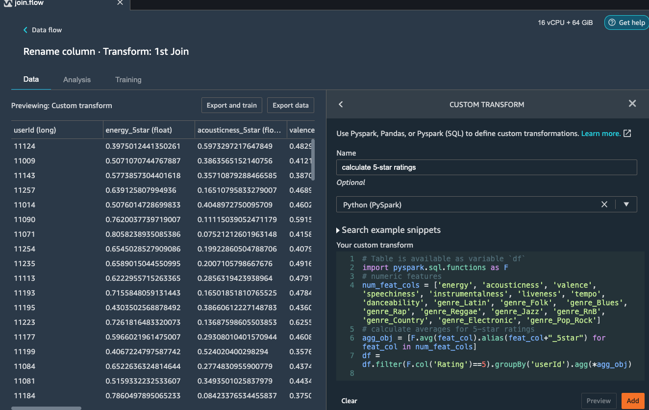
Click Preview and the Add this step to the flow.

We want to join the generated new features back to the original data. Before joining back, we notice some columns in the joint dataset are not needed for the model training, such as the id related columns. Let’s see now how to add a simple transform using Data Wrangler to drop the columns after the JOIN operation we did previously.

Select the jointrackid.csv block and select Add transform.

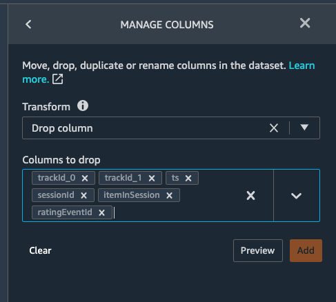
Let us apply the manage columns transform to drop some columns listed as below

trackId_0 trackId_1 ts sessionId itemInSession ratingEventId

image

we can drop multiple columns by selecting each column from the drop down manual.

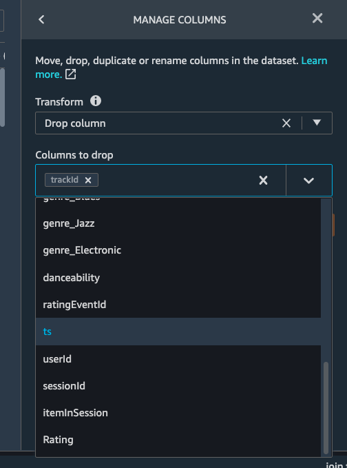
Once all the columns are selected, hit Preview first and then Add.

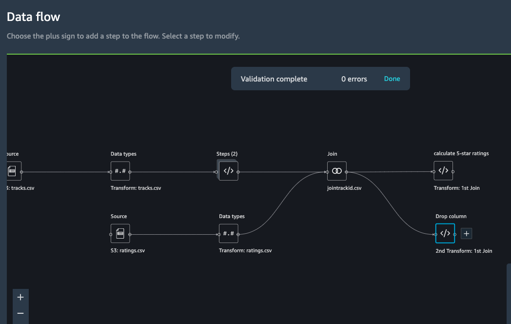
Now go back to data flow.

You should now be able to see the 2 transforms (custom transform and dropping the columns) as shown below in the Data Flow interface.

Next step is to join the two dataset back together. Similarly as the first join, we select one block and choose Join.

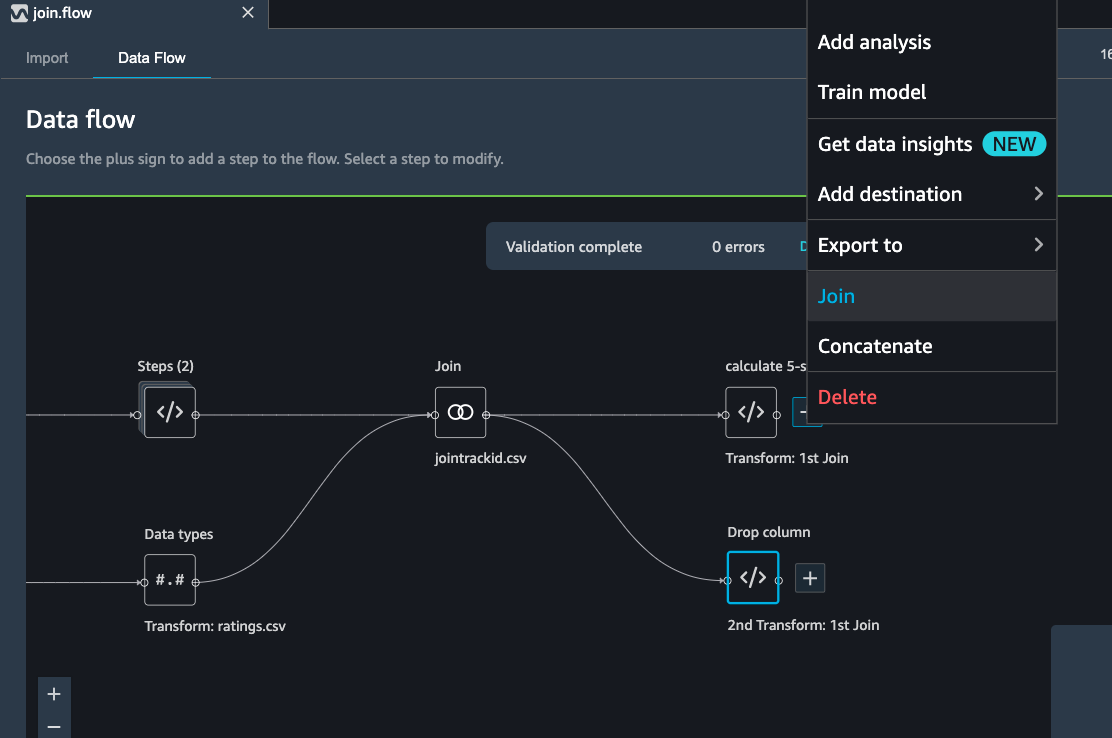
Select the other file transform block and get a Join preview.

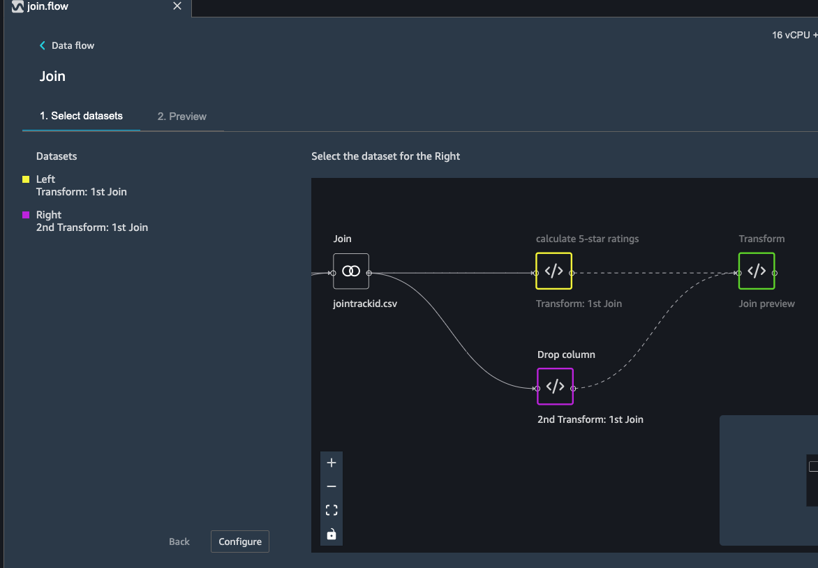
Fill in the step Name, Join Type and columns to join on (UserId).

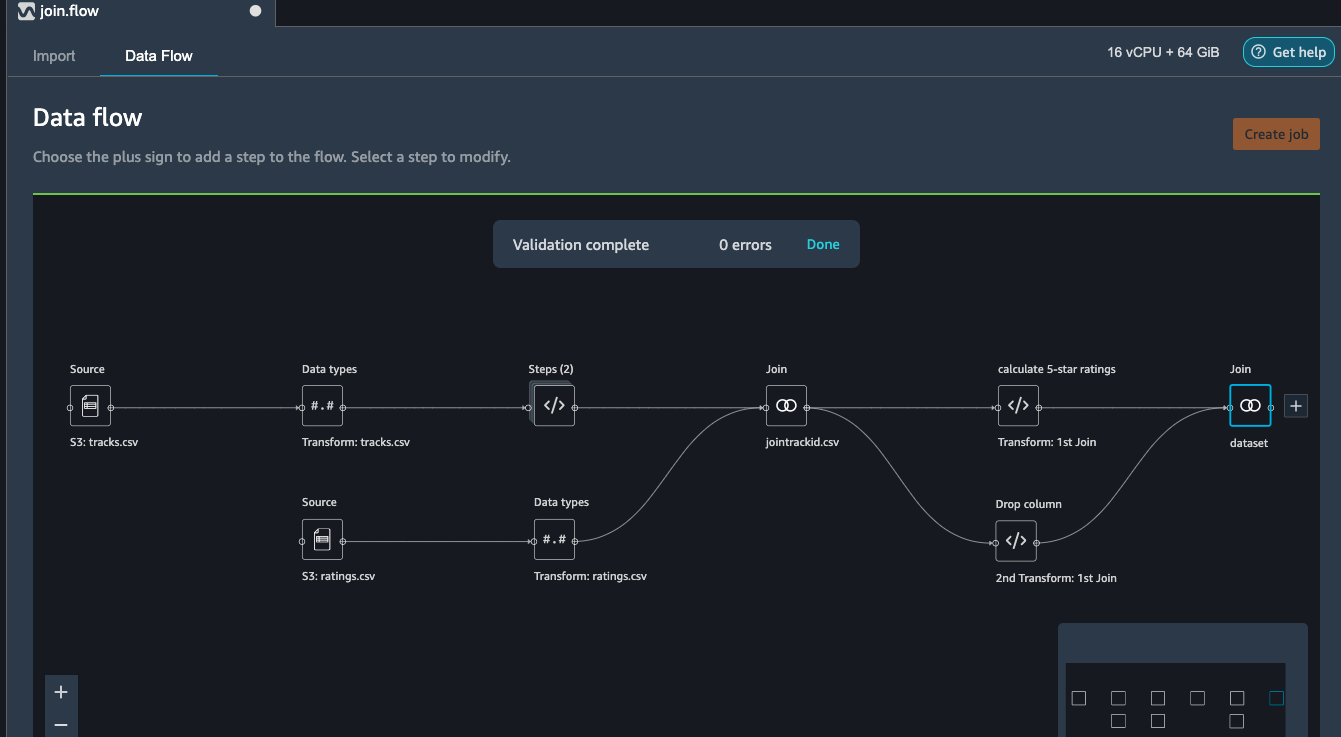
Preview and Add this step to the flow file. When we go back to the data flow, this is how the flow looks like now.

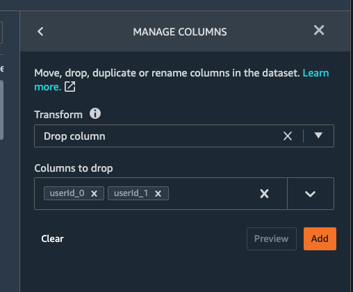
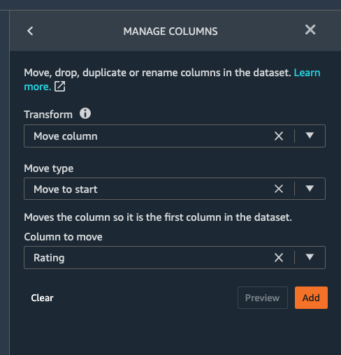
After joining the two data source, we also want to drop the userId columns and move the target column Rating to the first column.

Similar to the previous manage columns transform instructions, we add two transform steps to drop the userId_0 and userId_1 columns, and then move the Rating step to the start of the table.

Once all the transform steps are finished, we will export the transformed data. SageMaker Data Wrangler also allow you to split your dataset into train and test based on the ratio you set.

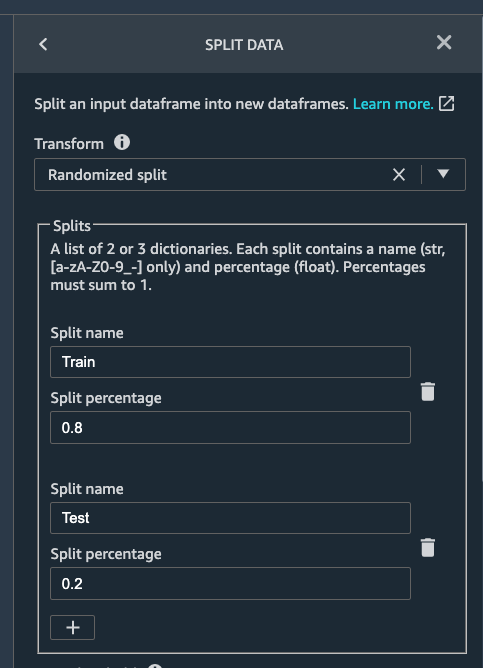
To split the dataset, add another transform step and choose Split data.

We choose Randomized split and get 80% for training and 20% data for testing.

The data flow now looks as below:

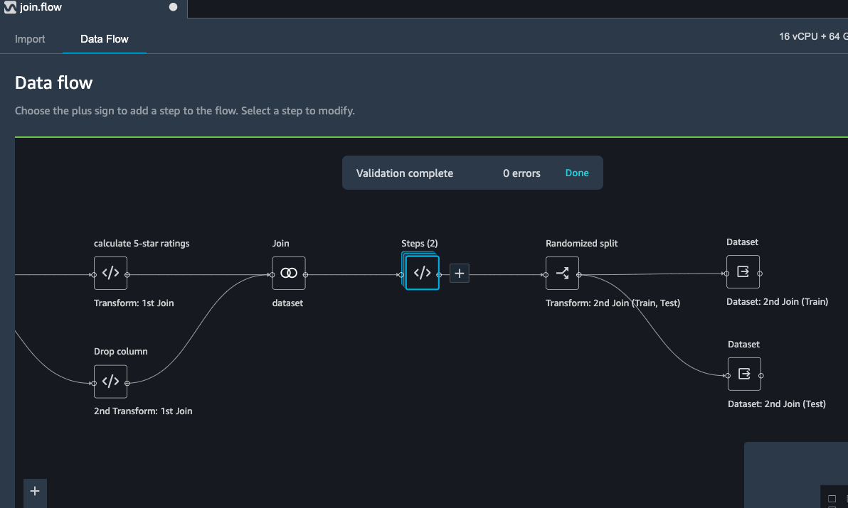
Export transformed features to S3

To export the transformed dataset, first click on the + symbol and choose Add Destination, followed by Amazon S3 as pointed out by the screen shot below.

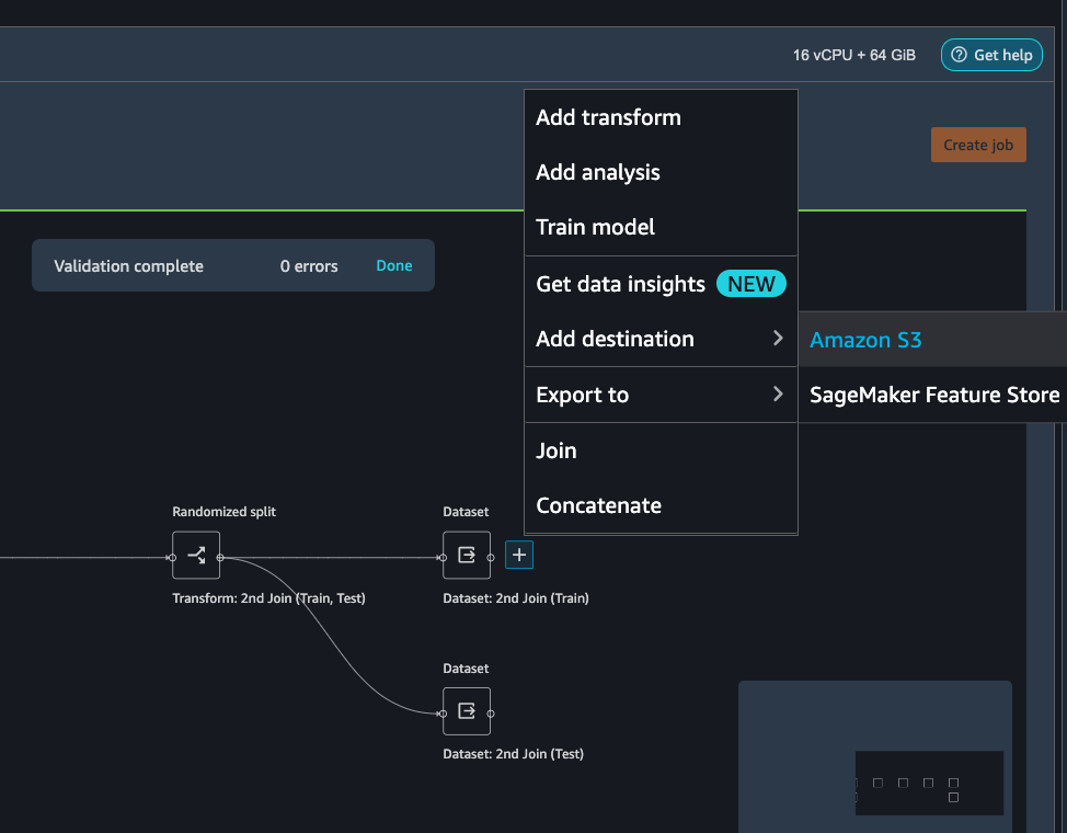
A new window is opened, Click Export data, choose the S3 location where you want to save the transformed dataset.

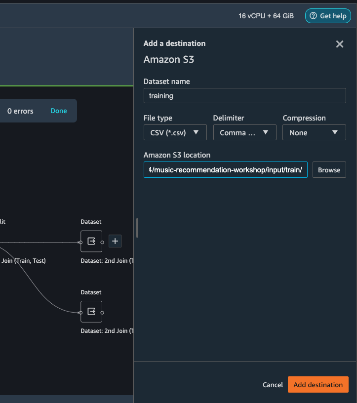
Follow the same step to set the S3 location for the test data.

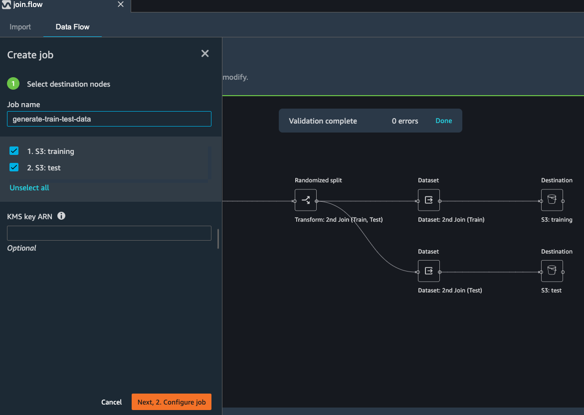
A job is needed to export the data to Amazon S3, to do this press the Create Job button on the top right, this will open a window.

Set the Job name to something like generate-train-test-data

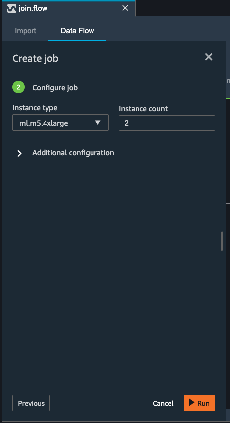
Hit the Configure Job button at the bottom

Leave the default instance type, and press the Run button at the bottom.

Note that your job has been created successfully and if you want to see the progress of the job you can do so by following the link to the generate-train-test-data process.

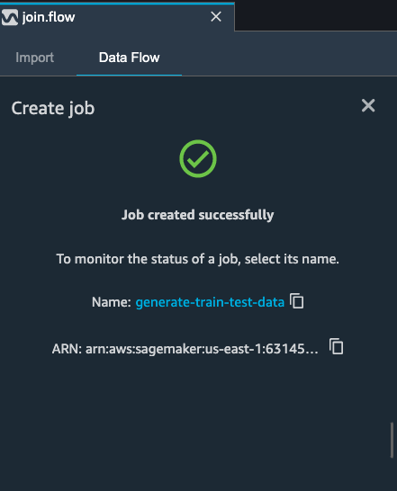
Follow the link to see the status of your job. This processing job takes around 5-10 mins.

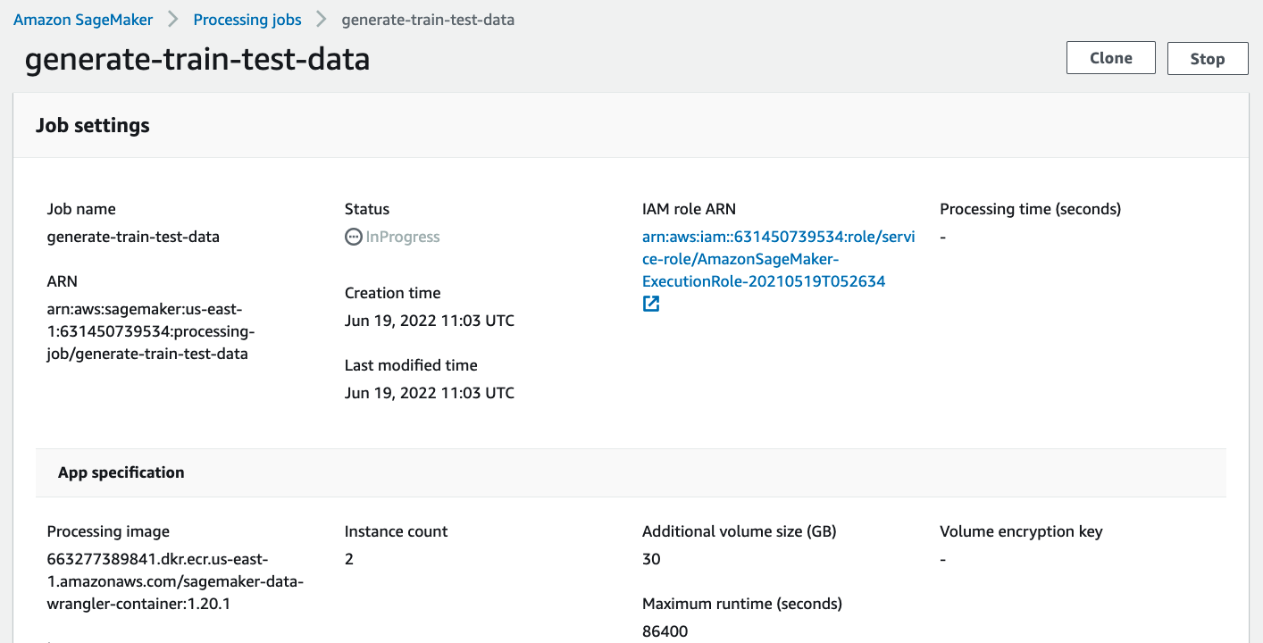
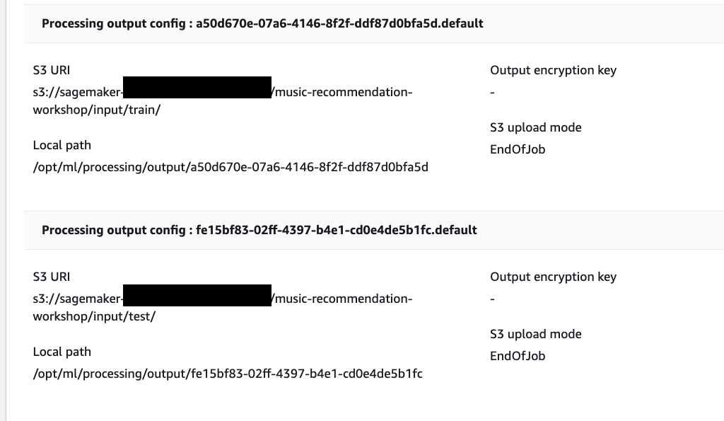
When the job is complete the train and test output files will be available in the corresponding S3 output folders. You can find the output location from the processing job configurations.

Other ways to export the transformations and analysis

The join.flow file that we created initially captures all of the transformations, joins and analysis.

In a way, this file allows us to capture and persist every step of our feature engineering journey into a static file.

The flow file can then be used to re-create the analysis and feature engineering steps via Data Wrangler. All you need to do is import the flow file to SageMaker Studio and click on it.

We saw previously, how to export transformed dataset into S3. Additionally, we can also export the analysis and transformations in many other formats.

To start exporting, click on the train Dataset data block and click on the + icon and select Export to.

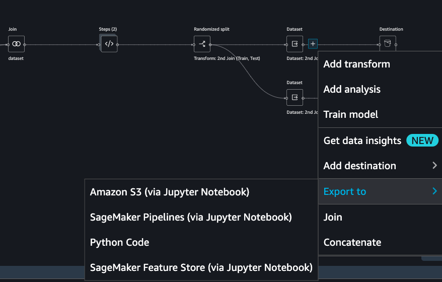
You can export the analysis and transforms in 4 different ways in addition to direct export to S3 which we saw previously.

• Save to S3 as a SageMaker Processing job notebook.

• Export as a SageMaker Pipeline notebook.

• Export as a Python script.

• Export to SageMaker Feature Store as a notebook.

So far, we have demonstrated how to use Amazon SageMaker Data Wrangler to preprocess the data and perform feature engineering to prepare for the train and test data set. After the data preparation step, data scientists can work on training a machine learning model using these datasets. In the next section, we will show you how to directly start a training job with the train data by leveraging Amazon SageMaker Autopilot from the SageMaker Data Wrangler data flow.

Import Dataflow

Here is the final flow file Flow file <https://github.com/aws/amazon-sagemaker-examples/sagemaker-datawrangler/joined-dataflow/join.flow> __

available which you can directly

import to expediate the process or validate the flow.

Here are the steps to import the flow

• Download the flow file

• In Sagemaker Studio, drag and drop the flow file or use the upload

button to browse the flow and upload

Optional : Run Autopilot training directly from Data Wrangler flow

SageMaker Data Wragler now allow you to directly run an Autopilot job to automatically train a model.

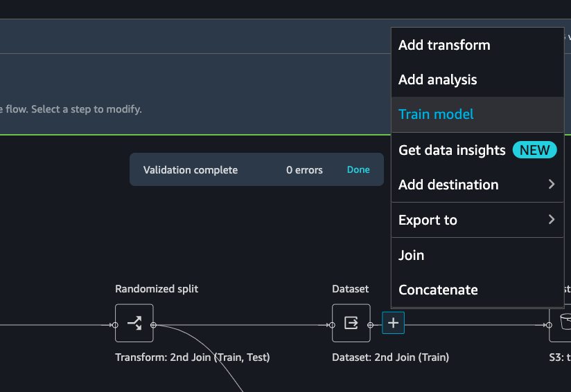
To set up a SageMaker Autopilot job, click the train data block, select Train model.

On the new window, select the S3 location you want the training dataset and the Autopilot job output to be saved.

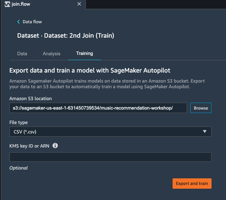
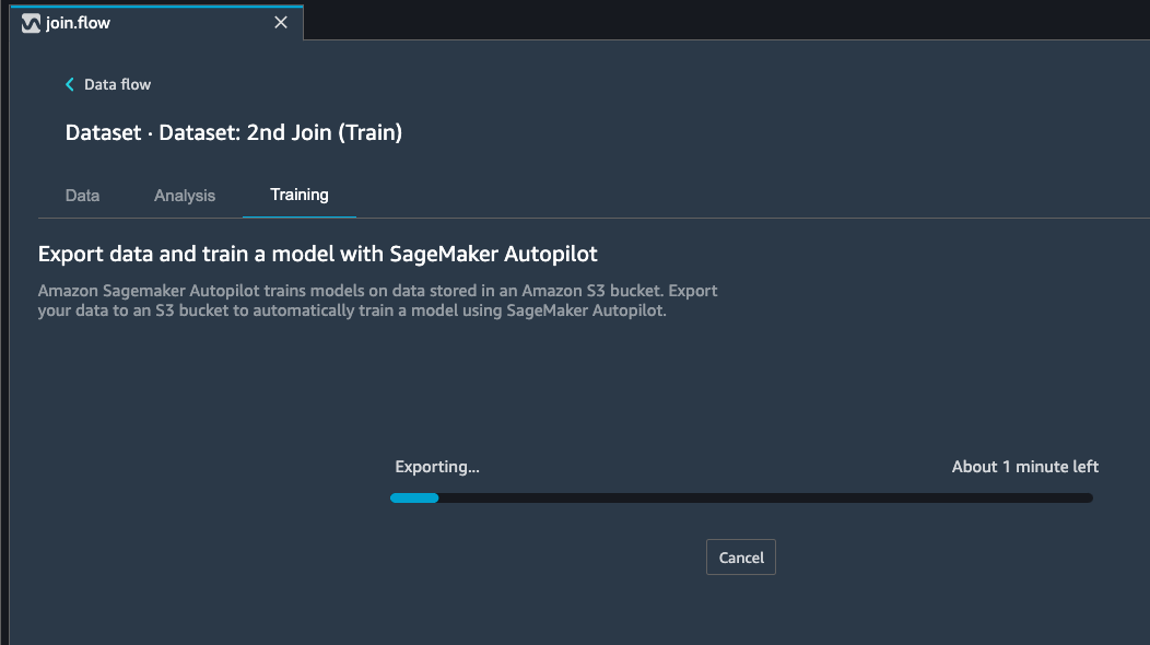
Select Export and train. This will take about one minute to export the train data to S3.

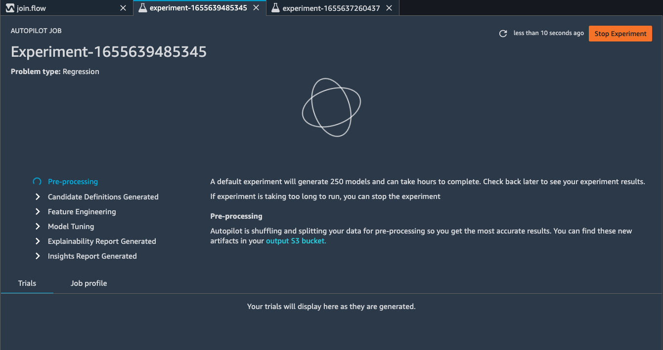
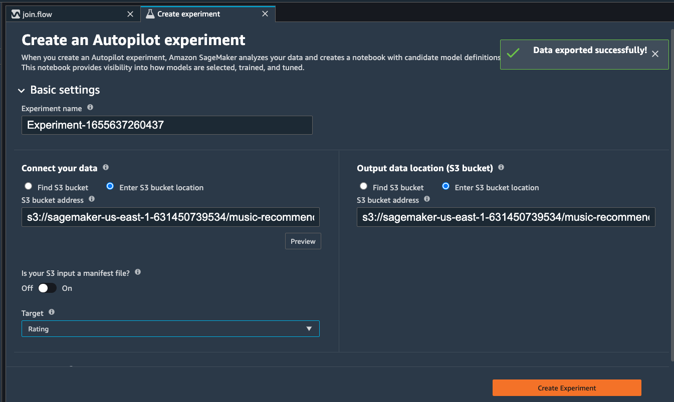
When data exported successfully, we can configure the Autopilot job. Select the Target training column (Rating).

Under the Advanced settings, choose the machine learning problem type as Regression. By default, SageMaker autopilot will run 250 training jobs to find the best model, this will take a few hours for the job to finish. To reduce runtime, you can set the Max candidates to a smaller number.

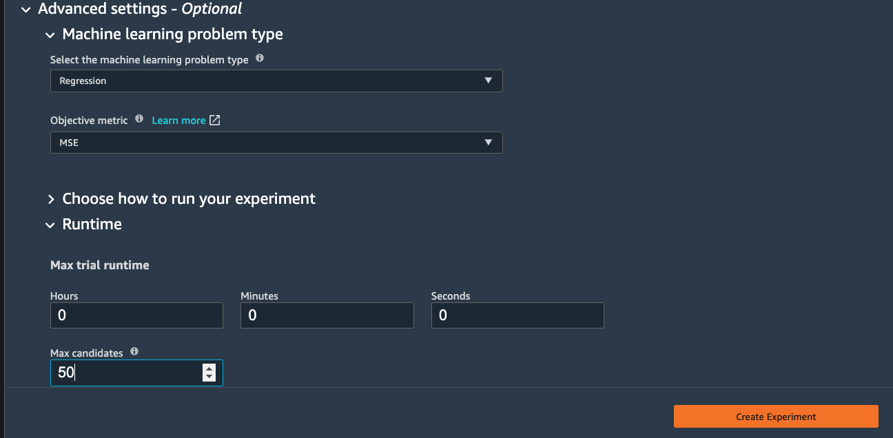
After click Create Experiment, an autopilot job will be started. You can come back to SageMaker Studio later to check the job output.